How I Learned Quick Sort!

I was first introduced to Quick Sort in my Algorithm's class at college. All that I could understand from my professor was that the algorithm used to select an element as a pivot and then sort all the elements around it. I could never wrap my head around how it worked and how I could implement it in my projects. So naturally, I skipped all my exam questions that were related to it and chose to forget its existance. But now, I decided to face my fears and finally tackle the quick sort problem and find out what made it so "quick". Here's how I set about doing so and ended up being super comfortable with it.

What is Quick Sort?

Quick Sort is a Divide and Conquer algorithm. It begins by picking an element from the list, called pivot and then re-arranges the rest of the elements in the list around this pivot to finally give us a sorted array.

How Does It Work?

The first step is to choose an element as a pivot from the array of unsorted elements. The pivot can be selected in any of the following ways:

• The first element of the array.
• The last element of the array.
• Any random element in the array.

After practicing for a while, I ended up choosing the first element as the pivot by habbit. I will stick to the same in this document.
Once the pivot is picked, it is placed at its sorted position in the array and the elements that are smaller than it in value are placed to its left, and those that are larger than it in value are placed to its right.

The heart of the Quick Sort algorithm is the patition function. The partition function returns the sorted position of the pivot element. Once the pivot is placed in its sorted position, the array is divided (partitioned) at this index and the quick sort algorithm is recursively applied to both the partitions. In the end, we are left with the entirely sorted array.
The pseudo code for the partition function is:

partition( low, high)
{
    pivot = A[ low ]
    i = low
    j = high

    while( i < j )
    {
        do
        {
            i++
        } while( A[i] <= pivot )
        
        do
        {
            j--;
        } while( A[j] > pivot )
        
        if ( i < j )
        {
            swap( A[i], A[j] )
        }
    }
    swap ( A[low], A[j] )
    return j;
}

A simplified explanation of this is:

• low is the first index which is an element and high is the highest index which has an element.
• i is assigned the value of low, j is assigned the value of high and pivot is assigned the value of A[low]
• Increment the value of i till we find a A[i] which is greater than pivot.
• Increment the value of j till we find a A[j] which is lesser than or equal to pivot.
• Once found, if i<j, swap the values of A[i] and A[j].
• Else if i>j, swap A[j] and A[pivot]. Thus, j is the sorted position of the pivot.
• Finally, the algorithm returns the value of j, which is now pointing to the sorted position of the pivot.
• The list is partition at the pivot sorted position and the QuickSort function is called recursively.

The pseudo code for the QuickSort() function is:

QuickSort( low, high)
{
    if ( low < high )
    {
        pivot_position = partition ( low, high)

        QuickSort( low, pivot_position )
        QuickSort( pivot_position + 1, high)
    }
}

Now, the working of the algorithm made a lot of sense to me and suddenly, I wasn’t so lost anymore. The next step was to put my knowledge to test by working with an example.

Let's Pair This With An Example!

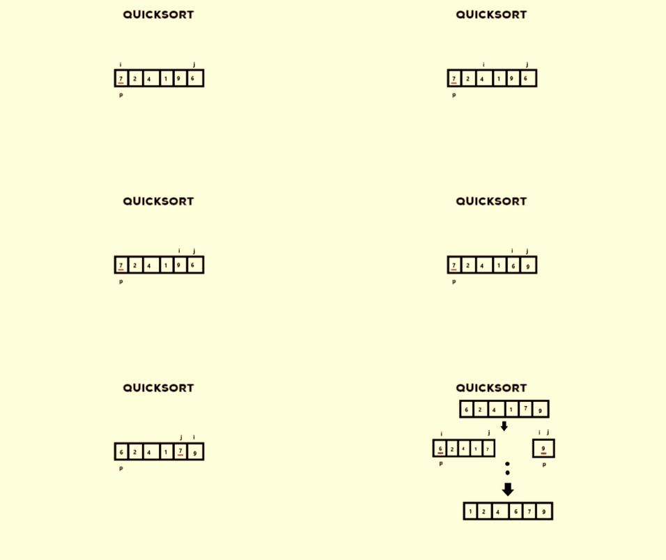
Let me show you the example that I worked on along with a single run of the partition function.

A = [ 7, 2, 4, 1, 9, 6 ]

pivot = 0 and A[ pivot ] = 7
i = 0
j = 5

-> i is incremented till we find A[i] > A[pivot]
    i = 4
    A[i] = 9

-> j is decremented till we find A[j] <= A[pivot]
    j = 5
    A[j] = 6

-> Here, i < j and so we swap A[j] and A[i]
    A[i] = 6    i = 4
    A[j] = 9    j = 5

-> Increment i till A[i] > A[pivot]
    i = 5
    A[i] = 9

-> Decrement j till A[j] <= A[pivot]
    j = 4
    A[j] = 6

-> This time, i > j, so swap A[j] and A[pivot]
    A[j] = 7    j = 4
    A[pivot] = 6    pivot = 0

-> The function returns j and then QuickSort is again 
    called on the arrays to the left and to the right of j.

If that’s too much of a head-scratcher, here’s a visualisation of what I have done.

Thank you for making it to the end of the post.
This is how I finally put in the time and effort to learn the workings of the Quick Sort algorithm which was initially a nightmare for me. I hope this blog helped you too.